Bayesian Neural Networks and Variational Dropout

Dmitry Mittov

• GitHub: @dmittov

• Twitter: @mittov

• Instagram: @mittov

• Company: Revolut

Plan

• Neural Networks: Recap
• Bayesian Machine Learning: Recap
• Bayesian neural networks
• Variational Dropout
• Conclusions

Neural Network (wrong)

Neural Network: MLP

Usual ML Task

We want to find the right \(\theta\):

\(y \approx f(X, \theta)\)

---

\(X\), \(y\) - data

\(y\) - targets: Data Scientists Salary

\(X\) - features: Python/Math skills, years of experience, etc

\(f\) - model, i.e. neural network

\(\theta\) - model parameters. weights of the network

Machine learning challenges

\(y \approx f(X, \theta)\)

• How to measure similarity?
• How to find weights?

Frequentist approach

• Similarity comes from the model of the error

\[ \forall{k} \quad y_k - f(X_k, \theta) \sim N(0, \sigma^2) \]

• Finding weights is method dependent
  • Stochastic gradient descent for Neural Networks
  • Can be found directly for Linear Regression

Maximum Likelihood

\[ y_k - f(x_k, \theta) \sim N(0, \sigma^2) \]

\[ p(y_k, x_k | \theta) = \frac{1}{\sqrt{2 \pi \sigma^2 }} e^{- \frac{1}{2} (\frac{y_k - f(x_k, \theta)}{\sigma})^2} \]

\[ \log p(y, X| \theta) \rightarrow \max \]

\[ \sum_k (y_k - f(x_k, \theta))^2 \rightarrow \min \]

Bayesian approach

\[ p(\theta | X, y) = \frac{p (y | X, \theta) \cdot p(\theta)}{p(X, y)} \]

\(p (y | X, \theta)\) - Likelihood from the frequentist approach

\(p(\theta)\) - prior distribution on model parameters

\(p(X, y)\) - data probability, we don’t know it

---

MAP: \(p(\theta | X, y) \rightarrow \max\)

Fair bayesian: \(\hat{y} = \mathbb{E}_{\theta} f(X, \theta)\)

MAP

\[ p(\theta | X, y) \rightarrow \max \]

\[ \hookrightarrow \log p(\theta | X, y) \rightarrow \max \]

\[ p(\theta | X, y) = \frac{p (y | X, \theta) \cdot p(\theta)}{p(X, y)} \]

\[ \log p(\theta | X, y) = \log p(y | X, \theta) + \log p(\theta) - C_1 \rightarrow \max \]

when we assume \(p(\theta) \sim N(0, \lambda)\):

\[ \sum(y_k - f(\theta, X_k))^2 + \lambda \sum \theta_j^2 \rightarrow \min \]

Interim conclusions

• Bayesian framework generalizes the frequentist’s approach

• When we simplify bayesian procedures, we get efficient techniques like regularization or ensembling

Dropout (picture)

Dropout (effect)

Dropout

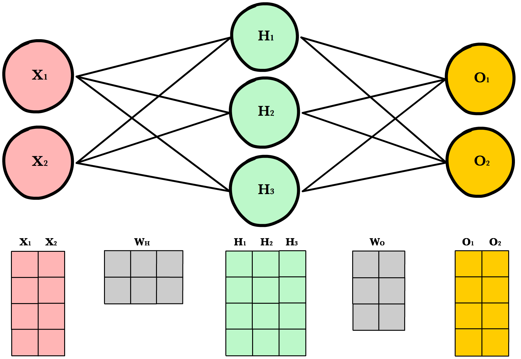
Data: \((X, y) = {(x_k, y_k)}_{k=1}^{N}\)

Network: \(p(y_k| x_k, \theta)\), where \(\theta\) - network parameters

SGD: \[ \theta_{t+1} = \theta_t - \gamma \frac{\partial \log p(y_k | x_k, \theta_t)}{\partial \theta_t}; \]

SGD with Dropout: \[ \theta_{t+1} = \theta_t - \gamma \frac{\partial \log p(y_k | x_k, \tilde{\theta_t})}{\partial \theta_t}; \quad \tilde{\theta_t} = \theta_t \cdot \epsilon \]

\[ \epsilon \sim Bernoulli(\epsilon | p); \quad \textrm{p - hyper-parameter} \]

Gaussian Dropout

SGD with Dropout: \[ \theta_{t+1} = \theta_t - \gamma \frac{\partial \log p(y_k | x_k, \tilde{\theta_t})}{\partial \theta_t}; \]

Classic: \[ \tilde{\theta_t} = \theta_t \cdot \epsilon \quad \epsilon \sim Bernoulli(\epsilon | p) \]

Gaussian: \[ \tilde{\theta_t} = \theta_t \cdot (1 + \epsilon) \quad \epsilon \sim N(\epsilon | 0, \sigma); \quad \sigma \textrm{ - hyper-parameter} \]

Dropout: Optimization target

\[ \mathbb{E} \frac{\partial \log p(y_k | x_k, \tilde{\theta})}{\partial \theta} = \int r(\epsilon) \sum_{k=1}^{N} \frac{\partial \log p(y_k | x_k, \theta (1 + \epsilon))}{\partial \theta} d\epsilon \]

\[ = \frac{\partial}{\partial \theta} \sum_k \int r(\epsilon) \log p(y_k| x_k, \theta (1 + \epsilon)) = \frac{\partial}{\partial \theta} \int r(\epsilon) \log p(Y | X, \theta (1 + \epsilon)) d\epsilon \]

\[ \tilde{\theta} \sim N(\theta, \sigma \theta^2) \sim N (\mu, \sigma \mu^2) \]

\[ \boxed{ \frac{\partial}{\partial \mu} \int q(\tilde{\theta} | \mu, \sigma) \log p (Y | X, \tilde{\theta}) d\tilde{\theta} \quad } \]

Similarities between different Dropout techniques

• Applying noise to the network weights prevents overfitting

• It’s not clear why this works

• There are 2 sources of noise in the gradient:
  • index \(\sim U(k | 1, N)\)
  • \(\epsilon\)

• How to pick hyper-parameters?

Bayesian Neural Network

We have a distribution over all possible weights.

\(y = \mathbb{E}_{\theta \sim p}f(X, \theta) = \int_\theta{f(X, \theta) p(\theta) d\theta}\)

Simplifications:

• All weights are independent:
  \(p(\theta| X, y) = \prod p(\theta_{ijl} | X, y)\)
• \(p(\theta_{ijl}| X, y)\) is some well known distribution
  i.e. \(p(\theta_{ijl} | X, y) = p(\theta_{ijl} | \phi_{ijl}) = N(\theta_{ijl} | \mu_{ijl}, \sigma_{ijl}^2)\)

%%{init: {"theme": "dark", "themeVariables": {"fontSize": "12px"}, "flowchart":{"htmlLabels":false}}}%%
flowchart LR
  Mu["Mu"] --> Phi("Phi")
  Sigma --> Phi
  Phi --> Theta("Theta")

Bayesian Neural Network: Example

---

\(y = \mathbb{E}_{\theta \sim p}f(X, \theta) = \int_\theta{f(X, \theta) p(\theta) d\theta}\)

---

• \(p = \frac{1}{6} \qquad \theta = (1.2, 2.5, 2.8)\)
• \(p = \frac{1}{6} \qquad \theta = (0.5, 1.7, 2.8)\)
• \(p = \frac{1}{3} \qquad \theta = (-1.5, 1.5, 0.8)\)
• \(p = \frac{1}{3} \qquad \theta = (0.5, 1.7, 2.8)\)

Evidence Lower Bound

Evidence: \(p(X, y) \approx p_{\theta}(X, y) = p(X, y | \phi)\)

---

\[ \log p(X, y| \phi) \]

\[ = \log \int {p(X, y, z | \phi) \frac{q(z)}{q(z)}dz} \]

\[ = \log \mathbb{E}_{q(z)} \frac{p(X, y, z | \phi)}{q(z)} \]

\[ \geq \mathbb{E} \log \frac{p(X, y, z | \phi )}{q(z)} - \textrm{ELBO} \]

Kullback-Leibler divergence

\[ KL(q(z) \ || \ p(z | X, y, \phi)) := \mathbb{E}_q \log \frac{q(z)}{p(z | X, y, \phi)} \]

\[ = \mathbb{E}_q \log q(z) - \mathbb{E}_q \log \frac{p(X, y, z | \phi)}{p(X, y | \phi)} = \log p(X, y | \phi) - \mathbb{E}_q \log \frac{p(X, y, Z | \phi)}{q(z)} \]

---

\[ \textrm{Evidence} = \textrm{ELBO} + \textrm{KL(q || p)} \]

\[ \textrm{Minimize KL divergence} \sim \textrm{Maximize ELBO} \]

Original Variational Dropout

\[ \textrm {Prior:} \quad p(\log(|\theta_{ijl}|)) = const \Leftrightarrow p(|\theta_{ijl}|) \propto \frac{1}{|\theta_{ijl}|} \]

\[ \textrm {Posterior:} \quad p(\theta | X, y) \approx q(\theta | \phi) = \prod_{ijl} N(\theta_{ijl} | \mu_{ijl}, \sigma^2) \]

\[ \hookrightarrow argmin_{\phi} KL( q(\theta | \phi) || p(\theta | X, y)) \rightarrow argmax_{\phi} ELBO \]

Gaussian Dropout is a specific case of Variational Inference

Improved Variational Dropout

\[ \textrm {Prior:} \quad p(\theta|\lambda) = \prod_{ijl} N(\theta_{ijl} | 0, \lambda_{ijl}^2) \]

\[ \textrm {Posterior:} \quad p(\theta | X, y) \approx q(\theta | \phi) = \prod_{ijl} N(\theta_{ijl} | \mu_{ijl}, \sigma_{ijl}^2) \]

• Tune \(\sigma\) for each parameter automatically
• Get rid of improper distribution \(\rightarrow\) normal prior distribution

Variational Dropout: ELBO

\[ argmin_{\phi = \{\mu, \sigma\}} KL(q(\theta | \phi) || p(\theta| X, Y)) = argmax_{\phi} ELBO \]

\[ = argmax_{\phi} \int q(\theta | \phi) \log p(Y| X, \theta) \frac{p(\theta)}{q(\theta | \phi)} d\theta \]

\[ = argmax_{\phi} \boxed{ \int q(\theta | \phi ) \log p(Y | X, \theta) d\theta \quad \\ data term } - \boxed{ KL(q(\theta | \phi) || p(\theta)) \quad \\ regularization } \]

\[ \frac{\partial}{\partial \mu} \int q(\theta | \mu, \sigma) \log p (Y | X, \theta) d\theta \quad \textrm{- Gaussian Dropout gradient} \]

Regularization term

Original Variational Dropout: \[ KL = func(\mu, \sigma) = func(\sigma) \]

ARD: Maximize ELBO by \(\mu, \sigma\) and \(\lambda\) \[ KL = \sum_{ijl} \left( \log \frac{\sigma_{ijl}}{\lambda_{ijl}} + \frac{\mu_{ijl}^2 + \sigma_{ijl}^2}{2 \lambda_{ijl}^2}\right) \]

\[ \lambda^{2 *}_{ijl} = \mu_{ijl}^2 + \sigma_{ijl}^2 \]

\[ KL = -\frac{1}{2} \sum_{ijl} \log \frac{\sigma^2_{ijl}}{\sigma^2_{ijl} + \mu_{ijl^2 }} + Const \]

ARD: Automatic Relevance Determination

\[ KL = -\frac{1}{2} \sum_{ijl} \log \frac{\sigma^2_{ijl}}{\sigma^2_{ijl} + \mu_{ijl^2 }} + Const \]

\[ \sigma_{ijl}^2 = \alpha_{ijl} \mu_{ijl}^2 \rightarrow q(\theta_{ijl} | \phi) = N (\theta_{ijl} | \mu_{ijl}, \alpha_{ijl} \mu_{ijl}^2) \]

\[ KL = -\frac{1}{2} \sum_{ijl} \log \frac{\alpha_{ijl}}{\alpha_{ijl} + 1} + Const \]

KL doesn’t depend on \(\mu\)

ARD: Effect

\[ q(\theta_{ijl} | \mu_{ijl}, \alpha_{ijl}) = N (\theta_{ijl} | \mu_{ijl}, \alpha_{ijl} \mu_{ijl}^2) \]

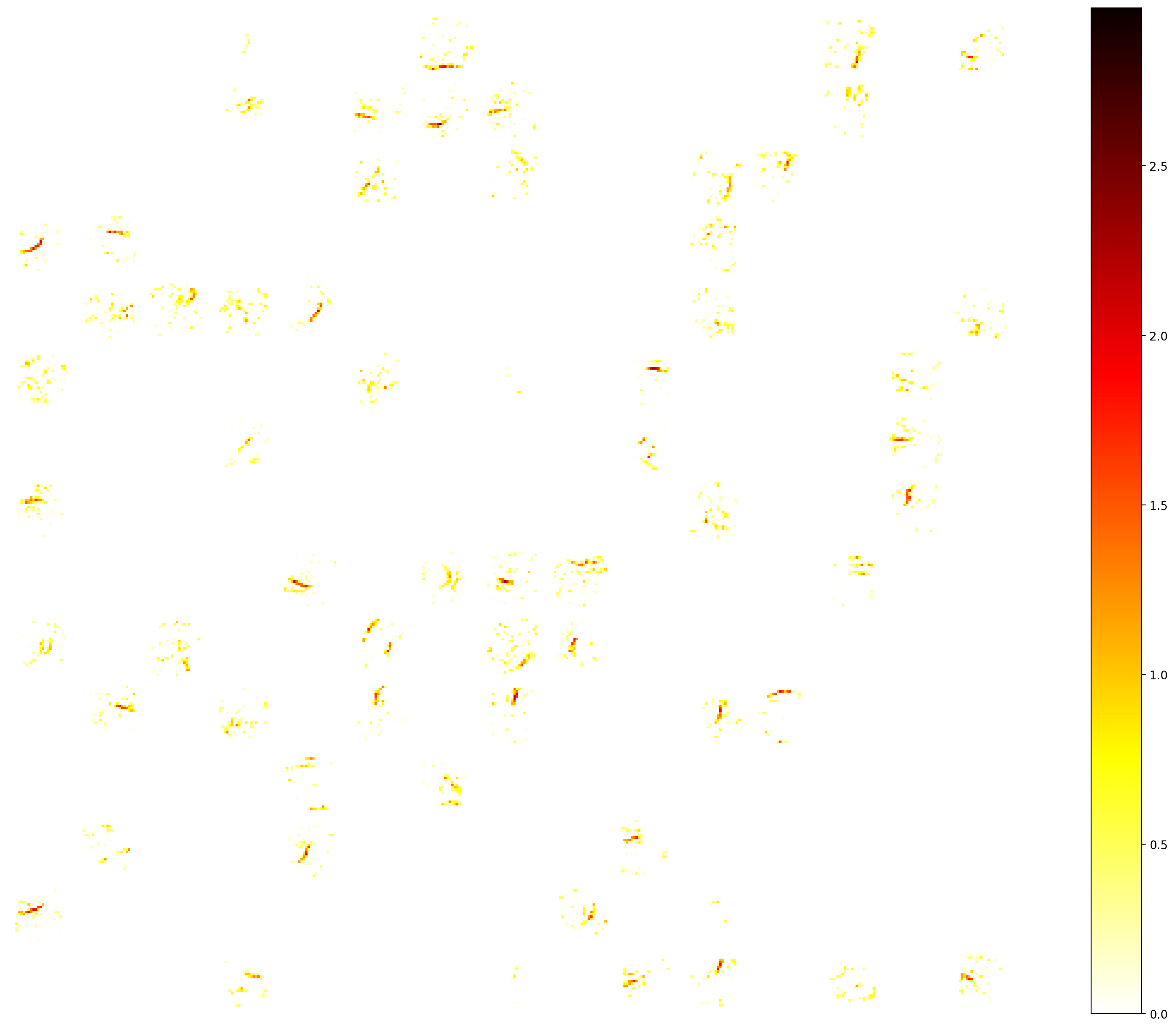
\[ \mu_{ijl} \rightarrow 0 \quad \textrm{and} \quad \alpha_{ijl} \mu_{ijl}^2 \rightarrow 0 \]

LeNet-300-100	Method	Error	Sparsity per Layer	Compression
	Original	1.64		1
	SparseVD	1.92	98.9 − 97.2 − 62.0	68

ARD: 35x compression

Data term: double stochastic estimation

\[ \frac{\partial \phi}{\partial} \int q(\theta | \phi ) \log p(Y | X, \theta) d\theta = \frac{\partial \phi}{\partial} \sum_{k} \int q(\theta | \phi) \log p(y_k | x_k, \theta) d\theta \]

\[ \theta = g(\phi, \epsilon) = \mu_{ijl} + \epsilon \sigma_{ijl} \quad \epsilon \sim N(\epsilon| 0, 1); \]

Use stochastic grad:

\[ \int r(\epsilon) \frac{\partial}{\partial \phi} \log p(y_k | x_k, g(\phi, \epsilon)) \]

MC estimation:

\[ \frac{\partial}{\partial \phi} \log p(y_k | x_k, g(\phi, \epsilon_s)) = \frac{\partial}{\partial g} \log p(y_k | x_k, g(\phi, \epsilon_s)) \frac {\partial g}{\partial \phi} \]

Training code

model = Net(threshold=3)
optimizer = torch.optim.Adam(model.parameters())
kl_weight = 0.00
epochs = 100

for epoch in tqdm(range(epochs)):
    model.train()
    kl_weight = min(kl_weight+0.02, 1)
    for batch_idx, (data, target) in enumerate(train_loader):
        data = data.view(-1, 28*28).float()
        optimizer.zero_grad()
        output = model(data)
        pred = output.data.max(1)[1] 
        loss = elbo(output, target, kl_weight)
        loss.backward()
        optimizer.step()

Model code

class Net(nn.Module):
    def __init__(self, threshold):
        super(Net, self).__init__()
        self.fc1 = LinearARD(28*28, 300, threshold)
        self.fc2 = LinearARD(300,  100, threshold)
        self.fc3 = LinearARD(100,  10, threshold)
        self.threshold=threshold

    def forward(self, x):
        x = F.relu(self.fc1(x))
        x = F.relu(self.fc2(x))
        x = F.log_softmax(self.fc3(x), dim=1)
        return x

ELBO code

class ELBO(nn.Module):
    def __init__(self, net, train_size):
        super(ELBO, self).__init__()
        self.train_size = train_size
        self.net = net
        self.loss = nn.NLLLoss()
        
    def forward(self, inputs, target, kl_weight=1.):
        kl = 0.
        for module in self.net.children():
            if hasattr(module, 'kl_reg'):
                kl += module.kl_reg()
        sz = inputs.shape[0]
        elbo_loss = self.train_size * self.loss(inputs, target) \
            + kl_weight * kl
        return elbo_loss 

Layer code

@property
def clip_mask(self):
    return 1 * torch.le(self.log_alpha, self.threshold)

def forward(self, x):      
    if self.training:
        self.log_mu = torch.log(torch.abs(self.mu) + self.eps)
        unstable_log_alpha = 2 * (self.log_sigma - self.log_mu)
        self.log_alpha = torch.clamp(unstable_log_alpha, -10, 10)
        
        # LRT
        lrt_mean = x @ self.mu.T
        clipped_sigma2 = torch.exp(self.log_alpha) * (self.mu ** 2)
        lrt_std2 = (x ** 2) @ clipped_sigma2.T
        lrt_std = (lrt_std2 + self.eps) ** .5

        epsilon = torch.normal(torch.zeros_like(lrt_mean), 
                                torch.ones_like(lrt_std))

        activation = lrt_mean + epsilon * lrt_std
        return activation + self.bias
    
    
    out = F.linear(x, (self.clip_mask * self.mu), self.bias)
    return out

def ard_reg(self):
    inv_alpha = torch.exp(-self.log_alpha)
    return 0.5 * torch.log1p(inv_alpha).sum()

Conclusions

• Bayesian framework generalized Dropout
• We can train not just weights, but also the variance of Gaussian Dropout (previously it was a hyper-parameter)
• We can tune variance for individual weights/neurons/layers
• We can sample ensembles from our bayesian neural network using just twice more weights

Follow-up papers

• 2017 Bayesian Sparsification of Recurrent Neural Networks Ekaterina Lobacheva, Nadezhda Chirkova, Dmitry Vetrov

• 2017 Structured Bayesian Pruning via Log-Normal Multiplicative Noise Kirill Neklyudov, Dmitry Molchanov, Arsenii Ashukha, Dmitry Vetrov

Links

Paper	Me